Guest Blog: Reproducible data pipelines in R with {targets}

In their tutorial on the targets package in R, Abner Bogan and Lindsay Platt share insights for the Earth Science Information Partners (ESIP) community. Abner and Lindsay are Environmental Data Scientists at the Consortium of Universities for the Advancement of Hydrologic Science, Inc. (CUAHSI ) — a nonprofit dedicated to advancing interdisciplinary water science.
Reproducibility is a huge challenge in science, especially as datasets grow larger and workflows become more complex. Enter targets — an R package that helps researchers create structured, automated data pipelines.
If you're juggling multiple datasets, collaborating with others or just tired of executing steps manually and remembering which scripts to rerun, targets can make your life easier.
This post breaks it down, from basic concepts to a practical implementation.
targets package at the January 2025 ESIP meeting (available on YouTube) and were invited to turn this into a guest blog post to make the resource more widely available.CUAHSI supports FAIR data practices by providing tools and training for reproducible workflows, making it easier for researchers to publish, access and collaborate on water data.
Learn more about CUAHSI’s data services and trainings at www.cuahsi.org or by contacting Lindsay (lplatt@cuahsi.org) or Abner (abogan@cuahsi.org) directly!
What’s the difference between a workflow and a pipeline?
A data workflow is the series of steps that turn raw data into something meaningful — think downloading, cleaning, analyzing and visualizing. You might already do this in R with a mix of scripts and notebooks. Some steps in your data workflow may also be manual and require no coding, such as data processing in Excel or uploading model output data to OneDrive.
A data pipeline, on the other hand, is an automated version of that workflow. It ensures that every step happens in order, only the necessary steps are rerun when data changes, and guarantees the results are reproducible every time. A well-structured pipeline ensures that anyone revisiting the analysis — including your future self — can rerun, verify and build on the work without extra effort or missing pieces.
Imagine what this looks like in a real-life scenario: You’re working on a project with a team, and you get a message from one of your colleagues — let’s say in this case me — some of the data you used needs to be updated.
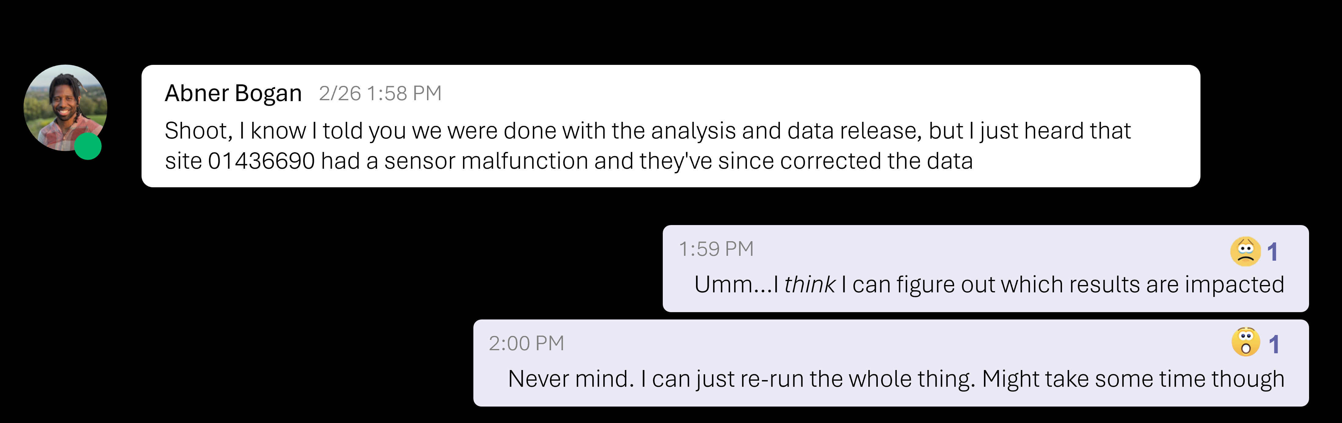
This kind of situation is common when a workflow relies on manual steps. Now you have to figure out which steps in your workflow are affected. Some parts are in R scripts, others were processed in Excel and maybe a teammate ran an analysis on their own computer.
Tracking down every step and making sure everything is updated correctly isn’t just tedious — it’s prone to errors and can be very stressful!
Now, imagine that you are managing this same data workflow using an automated pipeline. With a pipeline, any change you make to the underlying data or code will be appropriately propagated to downstream steps — meaning there is no need to manually rebuild everything or remember which components of the data analysis touch the updated data.
So if you had implemented a data pipeline, handling updates would be much simpler:

In short: Pipelines save time, reduce human error, and make it easier to collaborate!
And when it comes to reproducibility, pipelines are a powerful tool for conducting reproducible research — as defined in The Turing Way handbook, this means the same analysis run on the same data consistently and independently produces the same results.
Meet targets: a pipeline powerhouse for R
The targets package, developed by Will Landau, helps automate and organize R-based data workflows. It declares relationships between steps in the analysis and tracks dependencies, so that only the parts of your analysis that become outdated are rerun.
There are many types of pipelining tools (see this exhaustive list), but here’s what makes targets stand out:
- Designed specifically for R:
targetsis designed specifically for R, working seamlessly with its functional programming style for data science. It tracks dependencies and treats pipeline steps as R objects that can be readily inspected in the popular RStudio interactive development environment (IDE). - Uses interactive pipeline visualizations: Generates interactive dependency graphics to track and communicate pipeline structure.
- Improves project organization: Encourages writing modular code and implementing an organized file structure making projects easier to debug, maintain and collaborate on.
- Smarter execution: Instead of running everything from scratch,
targetsonly reruns what’s necessary, particularly helpful when running code with long execution times (e.g., models) and when frequent changes are made to code and data.
Moving from a function-based workflow to targets pipeline
Starting with functions is a great way to organize your workflow before making the leap to pipelines. If you're more used to script-based workflows — like basic R files or RMarkdown documents — getting more comfortable writing functions will equip you with a stronger base to take advantage of all the benefits of pipelining. For a deeper dive into transitioning from scripts to functions, check out these two blogs from the USGS Water Data For The Nation Blog Series: Writing Functions that work for you and Writing better functions.
At its core, a targets pipeline is a structured workflow made up of individual steps, known as “targets”. Each target represents a single output from performing a specific task — like a downloaded CSV file, a data.frame with missing values removed, or a scatter plot. The standard way to define a target is with the tar_target() function (from the targets library), which takes at least two key inputs: the target name and the function it runs.
The table below breaks down the three types of targets used in this tutorial, explaining how they are declared and when to use them.
Target type | Declaration | Examples |
|---|---|---|
Object |
| Anything that can be an R object (e.g., plots, models, data.frames) |
File |
| Files (e.g., csv or png output files) |
Dynamic |
| A series of object or file targets (e.g., a series of plots), one for each of the |
Let’s consider a more practical example to illustrate the difference between setting up a function-based workflow versus a targets pipeline. Say we have an example workflow with steps to read, clean, and plot data. The function-based workflow can be expressed in an R script called the run_model_workflow.R shown in the following section (adapted from the {targets} R package user manual):
# I named this file `run_model_workflow.R`
library(targets)
library(biglm)
source('R/myfunctions.R')

# Read and clean the data
data <- read_and_clean('data.csv')
fit <- fit_model(data)
hist <- create_plot(data)
The three functions called in this script are sourced from a file stored in the folder named “R” called myfunctions.R and then used in the last three lines of the run_model_workflow.R script. This workflow script can be executed by highlighting the entire script in the editor and pressing “Run” in the IDE to run the highlighted code.
We can express that same workflow as a targets pipeline (adapted from the {targets} R package user manual):
# This file must be named _targets.R
library(targets)
source('R/myfunctions.R')

tar_option_set(packages = c('biglm','tidyverse'))

list(
  tar_target(file,'data.csv', format = 'file'),
  tar_target(data, read_and_clean(file)),
  tar_target(model, fit_model(data)),
  tar_target(plot, create_plot(model, data))
)
In a targets pipeline, the file that controls the workflow is always called _targets.R and contains the recipe or instructions for how to execute the pipeline. The required libraries to execute the pipeline are defined in tar_option_set, and the steps in the workflow (we now know these are called targets!) are expressed as a list. The pipeline is executed by importing the targets library by running library(targets) in the console and then running the command tar_make().
That’s it—you have now officially seen a working targets pipeline!
Demoing utility of targets: automating water quality data workflows
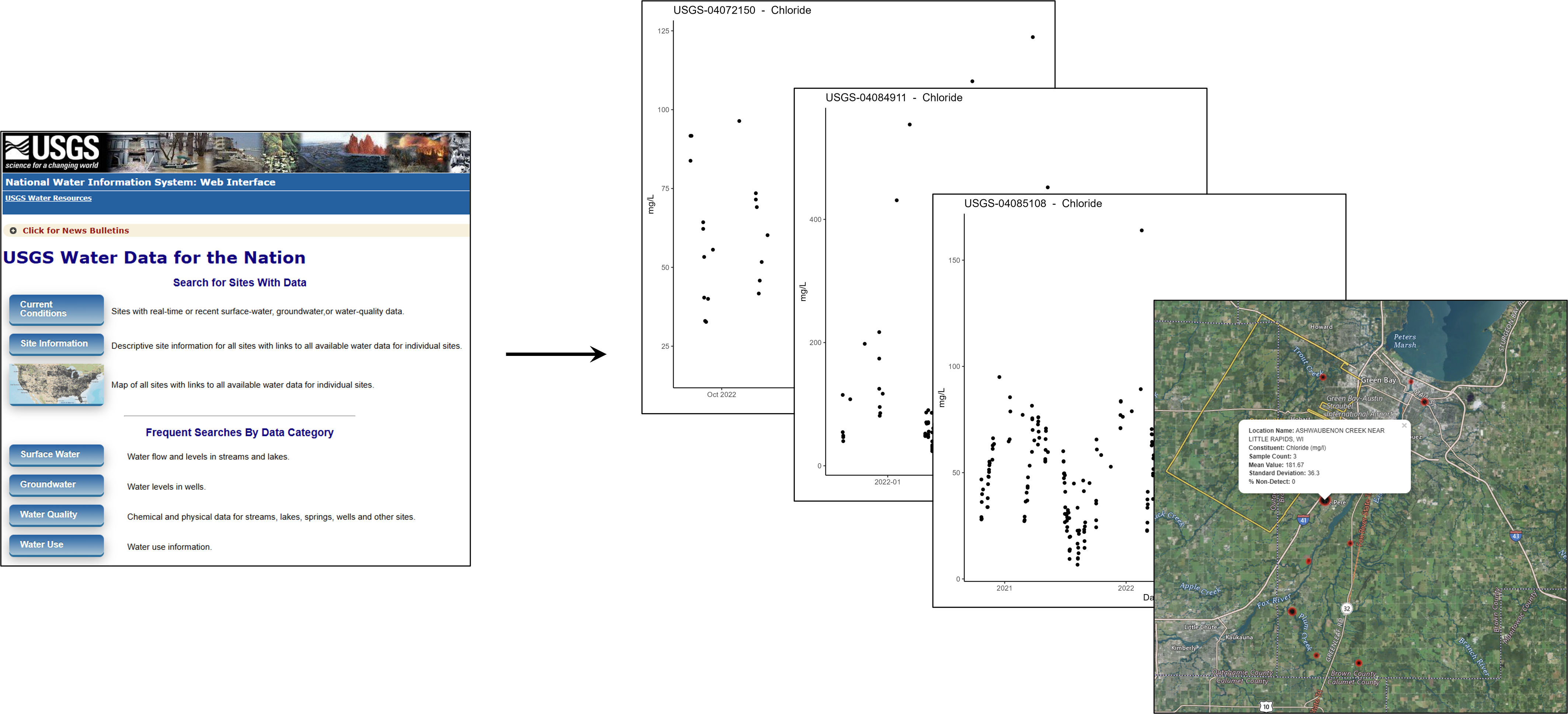
To illustrate in more detail how targets streamlines reproducible workflows, we built a pipeline that fetches water quality data from the Water Quality Portal, processes it for a single constituent of interest (e.g., nitrate), location, time range and generates visual summaries.
The pipeline, along with setup instructions and code, is freely available on ESIP Figshare. You can visit the page and download everything directly—no signup required! Try it out, explore the workflow and let us know how it works for you.
Want a guided walkthrough? Watch our presentation from the January ESIP meeting on YouTube, where we explore the contents in detail — jump straight to the relevant section with this timestamp!
Before executing the pipeline, let’s take a moment to review some key conventions observed that make it easier to maintain, debug, and collaborate on. First, let’s examine the folder structure.
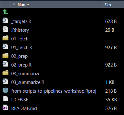
This pipeline follows a structured, phase-based approach:
- Folders are numbered to reflect execution order (e.g.,
01_fetch,02_prep). - Each phase has a corresponding individual target recipe file (e.g.,
01_fetch.R,02_prep.R).
While this organization and naming approach is not required by targets, it is recommended as a way to maintain organization and modularity. Before running the pipeline, it’s often good practice to inspect the workflow using tar_visnetwork(targets_only = TRUE). This function generates a dependency graph, providing a clear picture of the relationships between targets before execution. Note that the default visual often appears squished at first but you can drag each node vertically to space them out.
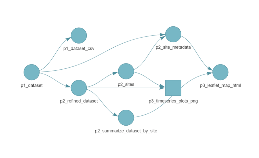
By viewing the pipeline, we can spot additional naming conventions that improve readability and organization:
- Target names reflect their phase (e.g.
p1_datasetindicates it belongs to Phase 1: fetching data). - File target names include a suffix for clarity (e.g.
p3_leaflet_map_htmlmakes it clear this target is an HTML file).
Now, let’s build the pipeline. First, load the targets package by running library(targets) and then execute the pipeline by running tar_make(). On the first run, every step in the pipeline will be executed. The console will display logs showing progress as each target is built. If you get errors right away, be sure to refer back to the installation instructions provided and make sure you installed all the necessary R package dependencies.
> library(targets)
> tar_make()
▶ dispatched target p1_dataset
GET: https://www.waterqualitydata.us/data/Result/search?profile=resultPhysChem&sampleMedia=water%3BWater&characteristicName=Chloride%3BPhosphorus%3BNitrate&statecode=US%3A55&countycode=US%3A55%3A009&startDateLo=10-01-2020&startDateHi=09-30-2023&mimeType=csv
GET: https://www.waterqualitydata.us/data/Station/search?profile=resultPhysChem&sampleMedia=water%3BWater&characteristicName=Chloride%3BPhosphorus%3BNitrate&statecode=US%3A55&countycode=US%3A55%3A009&startDateLo=10-01-2020&startDateHi=09-30-2023&mimeType=csv
NEWS: Data does not include USGS data newer than March 11, 2024. More details:
https://doi-usgs.github.io/dataRetrieval/articles/Status.html
● completed target p1_dataset [11.44 seconds, 123.298 kilobytes]
▶ dispatched target p2_refined_dataset
● completed target p2_refined_dataset [0.02 seconds, 29.207 kilobytes]
▶ dispatched target p1_dataset_csv
● completed target p1_dataset_csv [0.28 seconds, 2.608 megabytes]
▶ dispatched target p2_summarize_dataset_by_site
● completed target p2_summarize_dataset_by_site [0.02 seconds, 582 bytes]
▶ dispatched target p2_sites
● completed target p2_sites [0 seconds, 145 bytes]
▶ dispatched target p2_site_metadata
● completed target p2_site_metadata [0.02 seconds, 1.69 kilobytes]
▶ dispatched branch p3_timeseries_plots_png_32013e4d4bf87926
● completed branch p3_timeseries_plots_png_32013e4d4bf87926 [1.74 seconds, 50.883 kilobytes]
▶ dispatched branch p3_timeseries_plots_png_0f43ffdcd8385c9f
● completed branch p3_timeseries_plots_png_0f43ffdcd8385c9f [0.2 seconds, 52.287 kilobytes]
▶ dispatched branch p3_timeseries_plots_png_245c6024f5690fae
● completed branch p3_timeseries_plots_png_245c6024f5690fae [0.18 seconds, 65.38 kilobytes]
▶ dispatched branch p3_timeseries_plots_png_c4f30956531f1bee
● completed branch p3_timeseries_plots_png_c4f30956531f1bee [0.2 seconds, 61.396 kilobytes]
▶ dispatched branch p3_timeseries_plots_png_e968ff75b0269bbc
● completed branch p3_timeseries_plots_png_e968ff75b0269bbc [0.19 seconds, 62.271 kilobytes]
▶ dispatched branch p3_timeseries_plots_png_1d25049f1ab3a03e
● completed branch p3_timeseries_plots_png_1d25049f1ab3a03e [0.2 seconds, 73.894 kilobytes]
▶ dispatched branch p3_timeseries_plots_png_a1f76e7490770df3
● completed branch p3_timeseries_plots_png_a1f76e7490770df3 [0.21 seconds, 67.449 kilobytes]
▶ dispatched branch p3_timeseries_plots_png_8698411f1da8a6b5
● completed branch p3_timeseries_plots_png_8698411f1da8a6b5 [0.19 seconds, 66.109 kilobytes]
▶ dispatched branch p3_timeseries_plots_png_4f7fa9a103de7ea4
● completed branch p3_timeseries_plots_png_4f7fa9a103de7ea4 [0.18 seconds, 68.884 kilobytes]
▶ dispatched branch p3_timeseries_plots_png_ae1a677f719eb9d9
● completed branch p3_timeseries_plots_png_ae1a677f719eb9d9 [0.19 seconds, 66.283 kilobytes]
▶ dispatched branch p3_timeseries_plots_png_6665f473e5f31620
● completed branch p3_timeseries_plots_png_6665f473e5f31620 [0.22 seconds, 137.569 kilobytes]
▶ dispatched branch p3_timeseries_plots_png_5a86f3755a1f054b
● completed branch p3_timeseries_plots_png_5a86f3755a1f054b [0.18 seconds, 85.322 kilobytes]
▶ dispatched branch p3_timeseries_plots_png_5f3cb5e4e4ecb480
● completed branch p3_timeseries_plots_png_5f3cb5e4e4ecb480 [0.23 seconds, 71.477 kilobytes]
▶ dispatched branch p3_timeseries_plots_png_853a2a484c218724
● completed branch p3_timeseries_plots_png_853a2a484c218724 [0.2 seconds, 49.676 kilobytes]
● completed pattern p3_timeseries_plots_png
▶ dispatched target p3_leaflet_map_html
● completed target p3_leaflet_map_html [3.39 seconds, 505.887 kilobytes]
▶ ended pipeline [21.08 seconds]
We successfully ran the pipeline! Once the pipeline completes, the outputs (the Leaflet map and time series plots) will be available in the 03_summarize/out directory.
What happens when we rerun the pipeline? Let’s try running tar_make() again and observe what happens.
> tar_make()
✔ skipping targets (1 so far)...
✔ skipped pipeline [0.2 seconds]
This time, all targets are skipped — because nothing in the pipeline has changed. Targets only re-build when their inputs have been modified. However — what if we wanted to change the reported constituent of interest to chloride instead of phosphorus? In our _targets.R file, we can change the characteristic value to “Chloride.”
# Set 01_fetch pipeline configurations
start_date <- "2020-10-01" # Date samples begin
end_date <- "2023-09-30" # Date samples end
state <- 'Wisconsin'
county <- 'Brown'

# Set 02_prep pipeline configurations
characteristic <- "Chloride" # E.g., Phosphorus, Chloride, Nitrate
fraction <- "Dissolved"

source('01_fetch.R')
source('02_prep.R')
source('03_summarize.R')
Before running the pipeline, run the command tar_visnetwork(targets_only = TRUE) to visualize how the pipeline has been modified and what targets need to be updated.
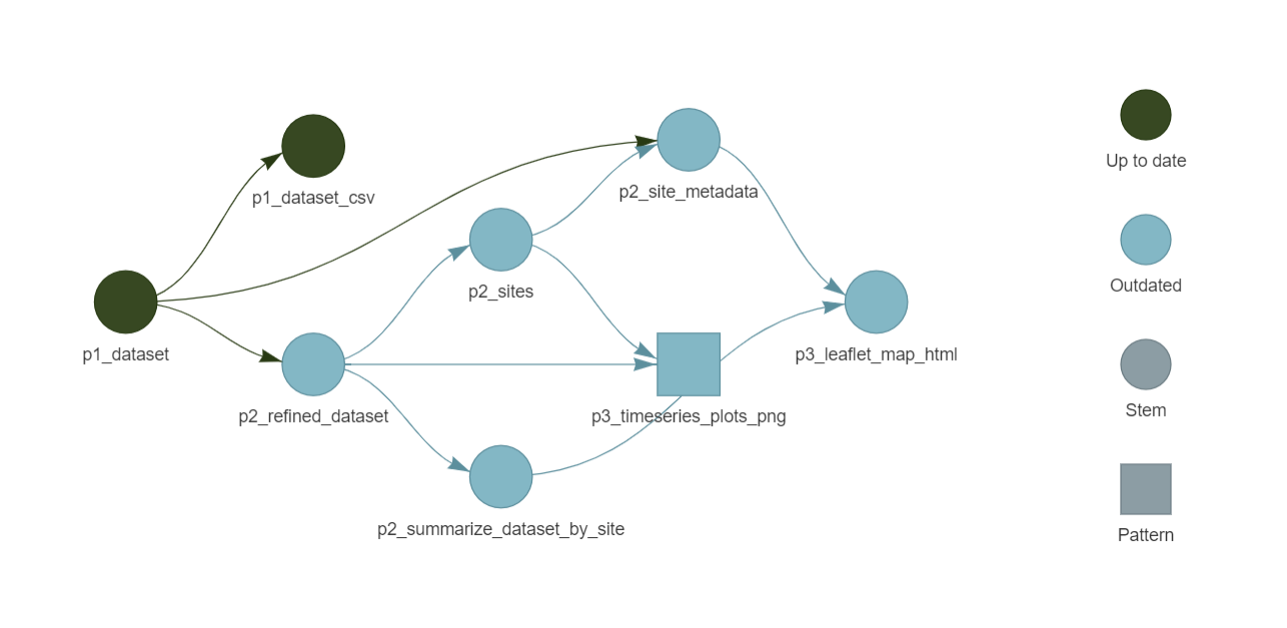
All of the blue shapes show targets that will be queued to rebuild the next time you run tar_make() because they depend on the change from ‘Phosphorus’ to ‘Chloride’. If at any point the data output at a target is the same as it was before the change, then the remaining targets in that dependency chain would be skipped. We can now run the pipeline and see the steps dependent on the p2_refined_dataset target rebuild (note in the logs how the p1_dataset target for data download is skipped).
> tar_make()
✔ skipping targets (1 so far)...
▶ dispatched target p2_refined_dataset
● completed target p2_refined_dataset [0.02 seconds, 30.872 kilobytes]
▶ dispatched target p2_summarize_dataset_by_site
● completed target p2_summarize_dataset_by_site [0.01 seconds, 431 bytes]
▶ dispatched target p2_sites
● completed target p2_sites [0 seconds, 93 bytes]
▶ dispatched target p2_site_metadata
● completed target p2_site_metadata [0.02 seconds, 1.385 kilobytes]
▶ dispatched branch p3_timeseries_plots_png_7df6a8832ecef8de
● completed branch p3_timeseries_plots_png_7df6a8832ecef8de [0.51 seconds, 81.635 kilobytes]
▶ dispatched branch p3_timeseries_plots_png_32013e4d4bf87926
● completed branch p3_timeseries_plots_png_32013e4d4bf87926 [0.26 seconds, 98.174 kilobytes]
▶ dispatched branch p3_timeseries_plots_png_0f43ffdcd8385c9f
● completed branch p3_timeseries_plots_png_0f43ffdcd8385c9f [0.25 seconds, 114 kilobytes]
▶ dispatched branch p3_timeseries_plots_png_245c6024f5690fae
● completed branch p3_timeseries_plots_png_245c6024f5690fae [0.26 seconds, 160.224 kilobytes]
▶ dispatched branch p3_timeseries_plots_png_c4f30956531f1bee
● completed branch p3_timeseries_plots_png_c4f30956531f1bee [0.22 seconds, 134.364 kilobytes]
▶ dispatched branch p3_timeseries_plots_png_5a86f3755a1f054b
● completed branch p3_timeseries_plots_png_5a86f3755a1f054b [0.19 seconds, 61.58 kilobytes]
● completed pattern p3_timeseries_plots_png
▶ dispatched target p3_leaflet_map_html
● completed target p3_leaflet_map_html [1.01 seconds, 503.713 kilobytes]
▶ ended pipeline [4.42 seconds]
Thanks to targets, only modified steps are re-run. So when we change the constituent of interest from phosphorus to chloride, the pipeline efficiently updates the affected outputs without running any prior steps (e.g. no re-downloading data).
targets recap!
Here’s a quick recap of what targets brings to the table:
- Automates Workflows – Eliminates manual steps by structuring your analysis into a pipeline where each step (target) runs only when needed.
- Optimizes Reproducibility – Tracks dependencies and ensures results stay updated, making it easier to rerun analyses without errors.
- Enhances Collaboration – Keeps workflows organized and transparent, so teams can work more efficiently and keep track of updates to data or code.
We hope this blog post has made you a fan of targets! For deeper dives on targets:
- Official
targetsdocumentation: https://books.ropensci.org/targets/ - Get started with the
targetsR package in four minutes: https://github.com/wlandau/targets-four-minutes - Enough
targetsto Write a Thesis: https://biostats-r.github.io/biostats/targets - Short course on the
targetsR package: https://github.com/wlandau/targets-tutorial
This blog was written by Abner Bogan (CUAHSI, abogan@cuahsi.org) in collaboration with Lindsay Platt (CUAHSI, lplatt@cuahsi.org) and with edits from Allison Mills from ESIP.
ESIP (Earth Science Information Partners) is a community dedicated to addressing environmental data challenges. Learn more at esipfed.org and sign up for the weekly ESIP Update for Earth Science data events, funding opportunities, and webinars.